Download Wolfram Mathematica for macOS

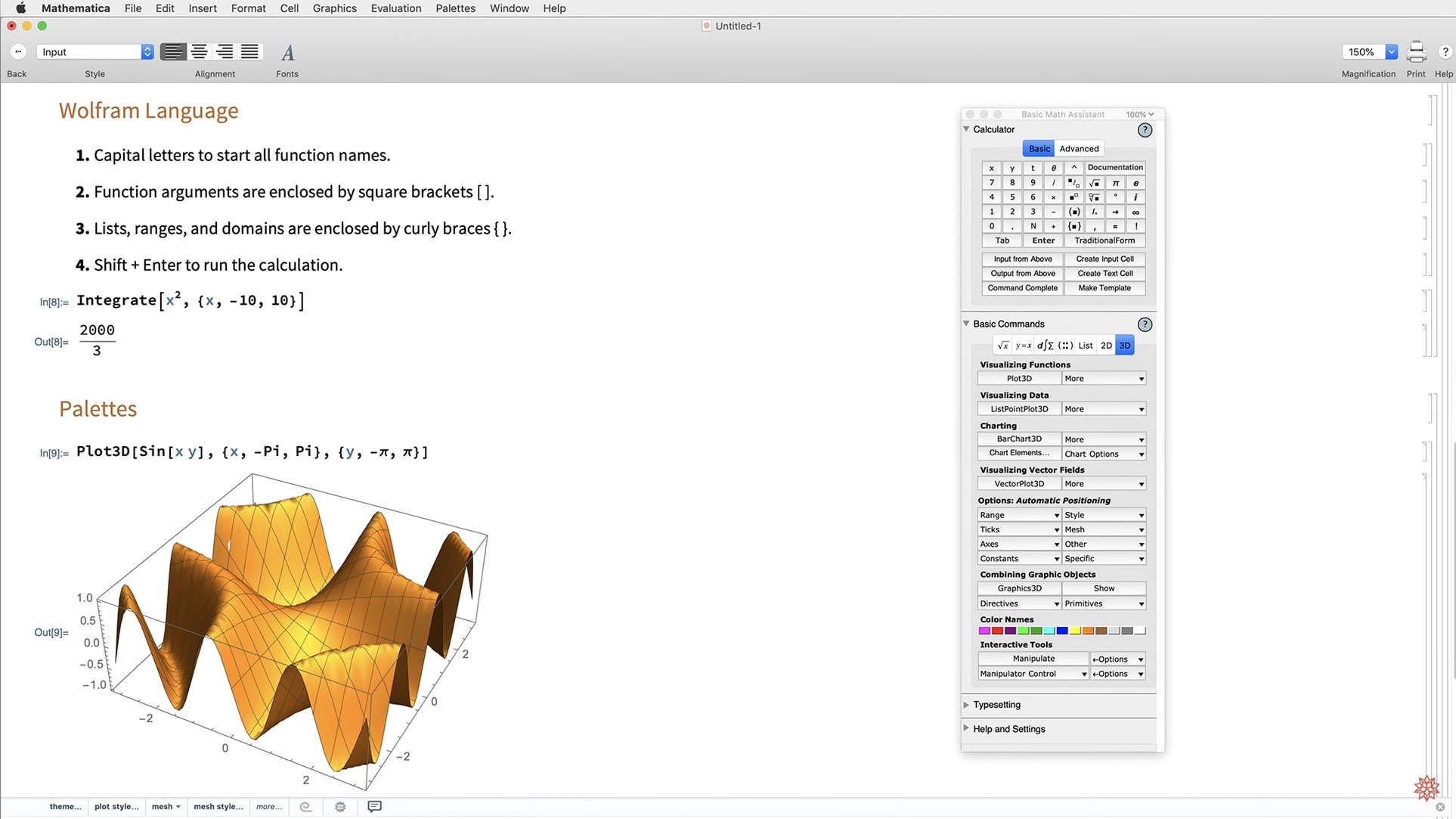
Getting a spreadsheet to handle advanced integrals or a plain Python script to produce publication-quality vector maps can feel like the tool is fighting back. Mathematica exists because those jobs need a platform that understands math, code, and visuals as parts of one conversation—often in plain English.

Reason from symbols and numbers

Whether it's simplifying a tough algebraic expression or running a high-speed numerical simulation on an Apple Silicon Mac, the engine treats both modes as first-class citizens. You can start with a formula, get an exact symbolic answer, then drop straight into a numeric approximation without switching tools.

Draw what the data means

Version 14.3 brings new surface plotting functions, ListFitPlot for fitting curves to points, and vector-based maps that scale cleanly for reports. Mesh processing tools help turn raw geometry into something you can inspect and share.

Connect to real-world pipelines

Pull in external data, run Python or R code with snappier integration than before, and validate system models right inside the notebook. When you're done, export to Markdown or deploy results in network-friendly formats—no extra conversion steps needed.

Where Mathematica fits on a Mac

Apple's ecosystem has a quiet strength when you pair Mathematica with it. The notebook interface plays nicely with Stage Manager on recent macOS versions, so you can keep a live computation on one side while drafting a report in Pages or laying out slides in Keynote on the other. Drag-and-drop of images and plain text works between apps without fuss. If you use iCloud Drive, storing notebooks there means a research session started on a MacBook Air picks up later on an iMac without manual syncing—just open the file.

Quick Look integration is a small but real timesaver. Tap the spacebar on a .nb file in Finder and you get a preview of the notebook content without launching the full application. For code-heavy workflows, the Wolfram Language kernel can run headlessly via Terminal, which slots into shell scripts, launchd jobs, and automated build pipelines the same way Python or R would.

Version 14.3's dark mode support arrived late but landed thoroughly—the new standard color set adjusts automatically, so plots and syntax highlighting stay readable whether your Mac is in light or dark appearance. No manual theme switching required.

Plain‑English integrals become symbolic results and plots

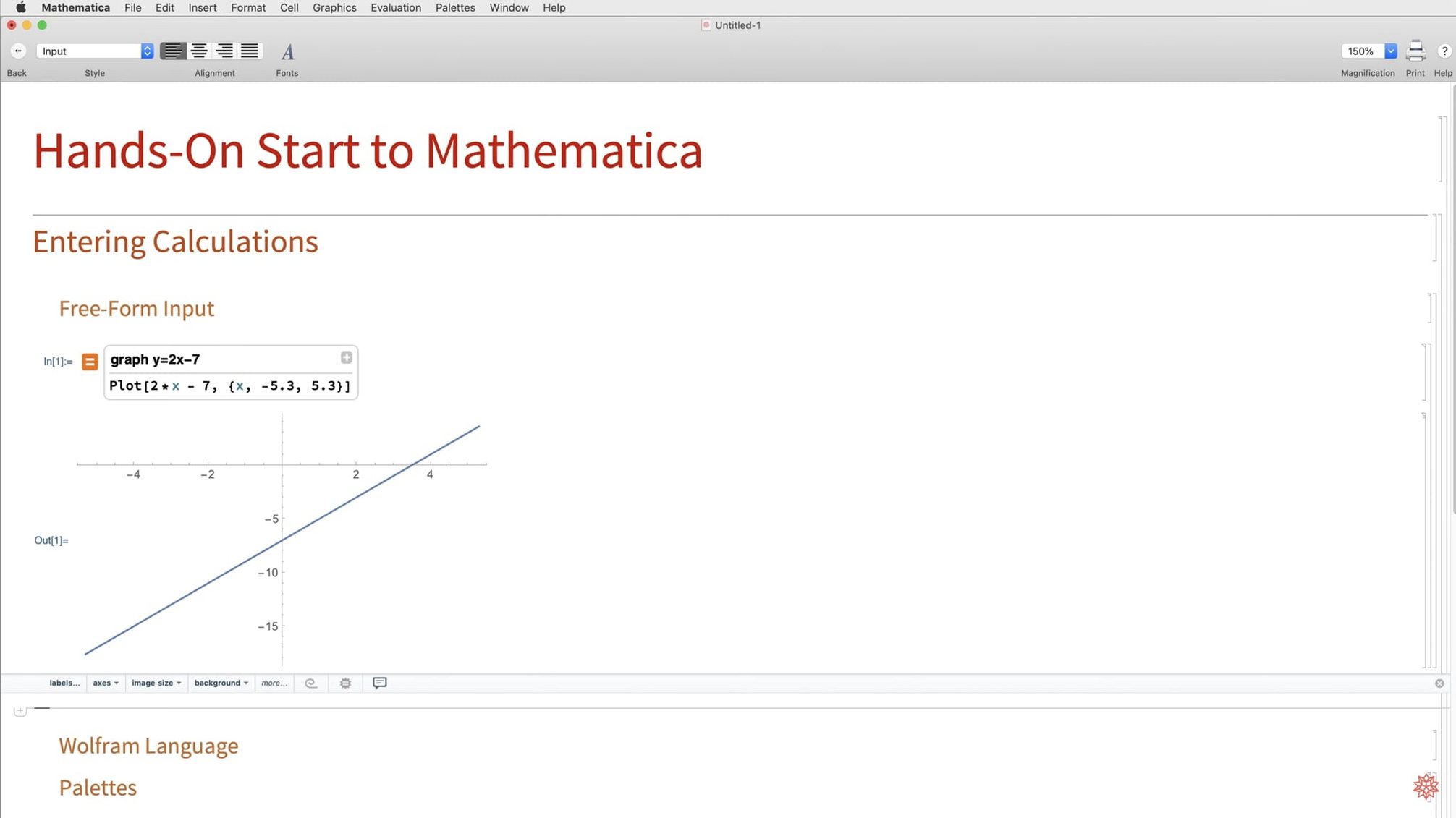
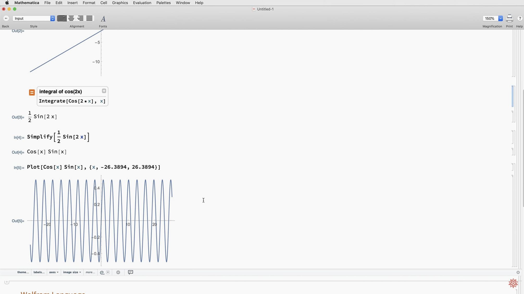
Undergraduate STEM students often discover Mathematica around their second year, when calculus and linear algebra problems outgrow a graphing calculator. The natural-language input means typing an integral in plain English can produce a symbolic result and a plot faster than wrestling with syntax you haven't fully learned yet.

Researchers in physics and engineering tend to stretch the tool further: symbolic manipulation of large expressions, control-system modeling with the new validation tools, and geodesic computations that feed into simulations. The expanded matrix decompositions in version 14.3 speak directly to anyone doing numerical linear algebra or data-driven modeling.

Data analysts and developers who already code in Python or R find Mathematica useful as an exploratory layer. The faster foreign-language integration means you can prototype a statistical model with Wolfram's visualization tools, then hand off the core logic to a Python script that runs in production. Architects and designers using mesh processing on imported 3D geometry also benefit—cleaning up scan data before export to a CAD tool is a workflow that fits naturally here.

Workflow: fitting and mapping experimental data

Say you have a CSV of temperature and pressure readings from a lab experiment, and you need a fitted curve overlaid on a clean vector map of sensor locations. Here's how it plays out start to finish.

First, import the data with a single command: data = Import["sensor_readings.csv"]. Mathematica typically detects headers and column types automatically. A quick ListPlot[data] confirms the raw scatter looks sensible.

Next, use the new ListFitPlot function to try a few models. Start with a linear fit to see the trend, then switch to a quadratic or a custom nonlinear model if the physics calls for it. The fitted curve overlays the data points directly, and the output includes residual statistics you can inspect before committing to a model.

For the sensor map, import latitude-longitude pairs and feed them into GeoListPlot. Version 14.3's vector-based maps render cleanly at any zoom level. Layer the fitted curve values as colored markers using a GeoRegionValuePlot, and the spatial pattern of the results becomes immediately obvious—hotspots jump out without additional annotation.

Finally, wrap everything in a single notebook with section headings, formatted text cells explaining the methodology, and the key plots inline. Export the whole thing to Markdown—new in version 14.3—and you have a self-contained document ready for a lab report or a team wiki. No screenshots, no separate image exports, and no last-minute formatting panic.

What's new in 14.3:

• Full support for dark mode, plus new standard colors tuned for light and dark environments.
• New visualization tools: ListFitPlot, surface plotting functions, vector-based maps, and mesh processing.
• Deeper math with Hilbert transforms, Lommel functions, and new matrix decompositions.
• Geodesic computation, LLMGraph, faster Python and R integration, ColumnwiseCombine, system model validation tools, and Markdown export support.

• macOS 12 or later
• Works on Apple Silicon and Intel 64-bit Macs